HoloViews 1.13 Release

release

holoviews

Release announcement for HoloViews 1.13

Author

Philipp Rudiger

Published

June 15, 2020

We are very pleased to announce the release of HoloViews 1.13.x!

Since we did not release blog posts for other 1.13 we will use this opportunity the many great features that have been added in this release. Note that this post primarily focuses on exciting new functionality for a full summary of all features, enhancements and bug fixes see the releases page in the HoloViews documentation.

Major features:

Add link_selection function to make custom linked brushing simple (#3951)
link_selection builds on new support for much more powerful data-transform pipelines: new Dataset.transform method (#237, #3932), dim expressions in Dataset.select (#3920), arbitrary method calls on dim expressions (#4080), and Dataset.pipeline and Dataset.dataset properties to track provenance of data
Add Annotators to allow easily drawing, editing, and annotating visual elements (#1185)
Completely replaced custom Javascript widgets with Panel-based widgets allowing for customizable layout (#84, #805)
Add HSpan, VSpan, Slope, Segments and Rectangles elements (#3510, #3532, #4000)
Add support for cuDF GPU dataframes, cuPy backed xarrays, and GPU datashading (#3982)
Add spatialpandas support and redesigned geometry interfaces for consistent roundtripping (#4120)
Add explicit .df and .xr namespaces to dim expressions to allow using dataframe and xarray APIs (#4320)

Other Features:

Support GIF rendering with Bokeh and Plotly backends (#2956, #4017)
Support for Plotly Bars, Bounds, Box, Ellipse, HLine, HSpan, Histogram, RGB, VLine and VSpan plots
Add support for linked streams in Plotly backend to enable rich interactivity (#3880, #3912)
Support for datashading Area, Spikes, Segments and Polygons (#4120)
HeatMap now supports mixed categorical/numeric axes (#2128)
Use __signature__ to generate .opts tab completions (#4193)

If you are using Anaconda, HoloViews can most easily be installed by executing the command conda install -c pyviz holoviews . Otherwise, use pip install holoviews.

Linked brushing

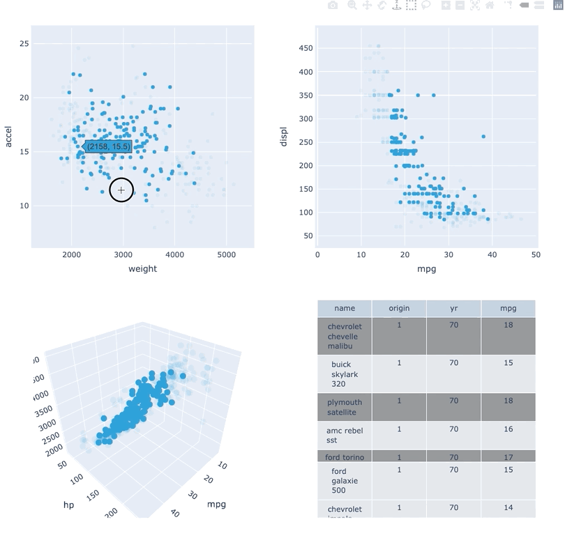
Datasets very often have more dimensions than can be shown in a single plot, which is why HoloViews offers so many ways to show the data from each of these dimensions at once (via layouts, overlays, grids, holomaps, etc.). However, even once the data has been displayed, it can be difficult to relate data points between the various plots that are laid out together. For instance, “is the outlier I can see in this x,y plot the same datapoint that stands out in this w,z plot”? “Are the datapoints with high x values in this plot also the ones with high w values in this other plot?” Since points are not usually visibly connected between plots, answering such questions can be difficult and tedious, making it difficult to understand multidimensional datasets. Linked brushing (also called “brushing and linking”) offers an easy way to understand how data points and groups of them relate across different plots. Here “brushing” refers to selecting data points or ranges in one plot, with “linking” then highlighting those same points or ranges in other plots derived from the same data.

In HoloViews 1.13.x Jon Mease and Philipp Rudiger worked hard on providing a simple way to expose this functionality in HoloViews by leveraging many of the existing features in HoloViews. The entry point for using this functionality is the link_selections function which automatically creates views for the selected and unselected data and indicators for the current selection.

Below we will create a number of plots from Gorman et al.’s penguin dataset and then applies the linked_selections function:

color_dim = hv.dim('Species').categorize({
    'Adelie Penguin': '#1f77b4',
    'Gentoo penguin': '#ff7f0e',
    'Chinstrap penguin': '#2ca02c'
})

scatter = hv.Scatter(penguin_ds, 'Culmen Length (mm)', ['Culmen Depth (mm)', 'Species']).opts(
    color=color_dim, tools=['hover']
)
bars = hv.Bars(penguin_ds, 'Species', 'Individual ID').aggregate(function=np.count_nonzero).opts(
    xrotation=45, color=color_dim
)
hist = penguin_ds.hist('Body Mass (g)', groupby='Species', adjoin=False, normed=False).opts(
    hv.opts.Histogram(show_legend=False, fill_color=color_dim)
)
violin = hv.Violin(penguin_ds, ['Species', 'Sex'], 'Flipper Length (mm)').opts(
    split='Sex', xrotation=45, show_legend=True, legend_position='right', frame_width=240,
    cmap='Category20'
)

hv.link_selections(scatter+hist+bars+violin, selection_mode='union').cols(2);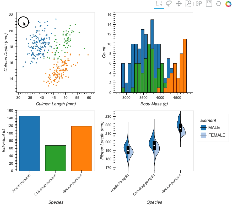

As we can see the linked selections functionality allows us to link a variety of plot types together and cross-filter on them using both box-select and lasso-select tools. However the real power behind the linked selections support is the fact that it allows us to select on the raw data and automatically replays complex pipelines of operations, e.g. below is a dashboard built in just a few lines of Python code that generates histograms and datashaded plots of 11 million Taxi trips and then links them automatically. In this way we can gain insights into large and complex datasets, e.g. identifying where Taxi trips departing at Newark airport in NYC drop off their passengers:

To read more about linked brushing see the corresponding user guide.

GPU support

The Rapids initiative started by NVIDIA has made huge strides over the last couple of years and in particular the cuDF library has brought a GPU backed DataFrame API to the PyData ecosystem. Since the cuDF and cupy libraries are now mature enough we developed a cuDF interface for HoloViews. You can now pass a cuDF DataFrame directly to HoloViews and it will leverage the huge performance gains when computing aggregates, ranges, histograms and thanks to the work of the folks at NVIDIA and Jon Mease you can now directly leverage GPU accelerated Datashader to interactively explore huge datasets with amazing latency, e.g. using the NYC taxi datasets you can easily achieve 10x performance improvements when computing histograms and datashaded plots further speeding up the dashboard presented above without changing a single line of HoloViews code - a cuDF behaves as a drop-in replacement for a Pandas or Dask dataframe as far as HoloViews is concerned.

Data pipelines

HoloViews has for a long time to declare pipelines of operations to apply to some visualization. However if the transform involved some complex manipulation of the underlying data we would have to manually unpack the data, transform it some way and then create a new element to display it. This meant that it was hard to leverage the fact that HoloViews is agnostic about the data format, in many cases users would either have to know about the type of the data or access it as a NumPy array, which can leave performance on the table or cause unnecessary memory copies. Therefore we added an API to easily transform data, which also supports the dynamic nature of the existing .apply API.

To demonstrate this new feature we will load an xarray dataset of air temperatures:

air_temp = xr.tutorial.load_dataset('air_temperature')
air_temp

q = pn.widgets.FloatSlider(name='quantile')

quantile_expr = hv.dim('air').xr.quantile(q, dim='time')
quantile_expr

Seeing that this dataset has an 'air' variable we can write a so called dim expression to express a transform which performs a quantile quantile aggregation along the 'time' dimension:

q = pn.widgets.FloatSlider(name='quantile')

quantile_expr = hv.dim('air').xr.quantile(q, dim='time')
quantile_expr

dim('air').xr.quantile(FloatSlider(name='quantile'), dim='time')

As you can see the slider we have created is a valid argument to this transform and if we now apply this transform the pipeline is reevaulated whenever the slider value changes:

temp_ds = hv.Dataset(air_temp, ['lon', 'lat'])

transformed = temp_ds.apply.transform(air=quantile_expr).apply(hv.Image)

pn.Column(q, transformed.opts(colorbar=True, width=400))

In this way we can build transformation pipelines using familiar APIs (pandas or xarray) without losing the ability to inject dynamic parameters driven by widgets or other sources. To read more about data pipelines see the Transforming Elements and Data Processing Pipelines user guides.

Annotators

This release also introduced annotating functionality which allows editing, adding and labelling different a range of element types. At the moment it is possible to annotate the following element types:

Points/Scatter
Curve
Rectangles
Path
Polygons

As an example we will create a set of Points and use the annotate function to enable the annotator functionality:

cells = hv.Image(calcium_array[:, :, 0])

points = hv.Points([(-0.275, -0.0871875), (-0.2275, -0.1996875), (0.1575, 0.0003125)]).opts(
    padding=0, aspect='square', frame_width=400, responsive=False, active_tools=['point_draw']
)

annotator = hv.annotate.instance()

hv.annotate.compose(cells, annotator(points, name='Cell Annotator', annotations={'Label': str}))

If you select the PointDraw tool from the toolbar you will now be able to add new points, drag existing points around and edit their position and labels via the table. Once we are done we can access the edited data on the annotator object:

annotator.annotated.dframe()

	x	y
0	-0.2750	-0.087188
1	-0.2275	-0.199687
2	0.1575	0.000313

New elements

The addition of new visual elements always increases the power of a plotting library significantly. In this a number of elements were added to draw specific geometries and annotate plots.

Rectangles & Segments

The ability to draw rectangles and segments provides powerful low-level primitives to render higher-level plots, e.g. below we can see an OHLC plot, usually used to indicate the movement of stocks over time, generated using the new Rectangles and Segments elements:

def OHLC(N):
    xs = np.arange(N)
    ys = np.random.randn(N+1).cumsum()

    O = ys[1:]
    C = ys[:-1]
    H = np.max([O, C], axis=0) + np.random.rand(N)
    L = np.min([O, C], axis=0) - np.random.rand(N)
    return (xs, ys, O, H, L, C)

xs, ys, O, H, L, C = OHLC(50)
boxes = hv.Rectangles((xs-0.25, O, xs+0.25, C))
segments = hv.Segments((xs, L, xs, H))

# Color boxes where price decreased red and where price increased green
color_exp = (hv.dim('y0')>hv.dim('y1')).categorize({True: 'green', False: 'red'})

boxes.opts(width=1000, color=color_exp, xlabel='Time', ylabel='Price') * segments.opts(color='black')

HSpan and VSpan

The ability to draw shaded regions with unlimited extent allows highlighting notable regions along the x- or y-axis of a plot. The new HSpan and VSpan annotation elements allow you to do exactly that, here we mark the regions of the timeseries that are one standard deviation above and below the mean:

ys = np.random.randn(1000).cumsum()

ymean, ystd, ymin, ymax = ys.mean(), ys.std(), ys.min(), ys.max()

timeseries = hv.Curve(ys)

timeseries * hv.HSpan(ymean+ystd, ymax) * hv.HSpan(ymean-ystd, ymin)

Slope

Another helpful annotation is the ability to draw an infinite sloping line on a plot, complementing the existing HLine and VLine elements. The Slope element can be used to display a regression line for example:

scatter = penguin_ds.to(hv.Scatter, 'Body Mass (g)', 'Flipper Length (mm)', 'Species').overlay()

scatter * scatter.apply(hv.Slope.from_scatter, per_element=True).opts(legend_position='bottom_right', frame_width=400)

Panel based widgets

HoloViews has shipped with a set of widgets to explore multi-dimensional parameter spaces since its first public release. These widgets were written as a weekend project and did not follow many of the best practices of Javascript development. This meant they were hard to extend, exhibit a variety of issues related to character encoding and were not at all customizable. In HoloViews 1.13.0 we completely replaced most of the rendering machinery and widget code with Panel widgets making them easier to maintain, customize and extend.

Specifically so far the widgets have always been located at the right of a plot, but now we have full flexibility to override this:

calcium_hmap = hv.HoloMap({i: hv.Image(calcium_array[:, :, i]) for i in range(10)}, 'Time')

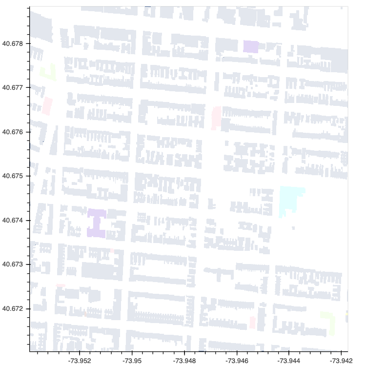
hv.output(calcium_hmap, widget_location='bottom')

Spatialpandas and polygon datashading

HoloViews has long had strong support for both gridded and tabular data, with geometry data support being more spotty. In HoloViews 1.13.0 the core model around support for geometry data was redesigned from the ground up, in particular HoloViews can now convert natively between different geometry storage backends including the native dictionary format, geopandas (if GeoViews is installed) and the new addition called spatialpandas. Spatialpandas is closely modeled on GeoPandas but does not have the same heavy GIS dependencies and is highly optimized, efficiently make use of pandas extension arrays. All of this means that spatialpandas is significantly more performant than geopandas and can also be directly ingested into datashader, making it possible to render thousands or even millions of geometries, including polygons, very quickly.

nyc_buildings = hv.Polygons(buildings, ['x', 'y'], 'type')

datashade(nyc_buildings, aggregator=ds.by('type', ds.count()), color_key=glasbey);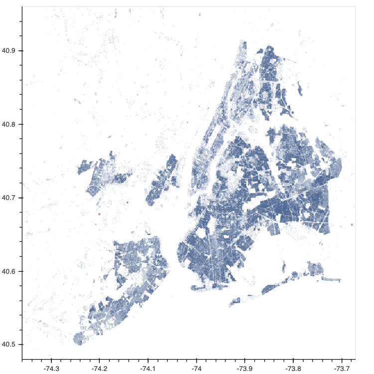

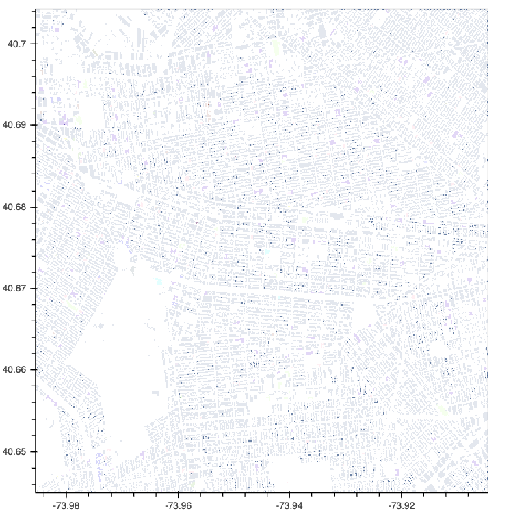
In addition to Polygons this release also brings support for datashading a range of other plot types including Area, Spikes and Segments:

xs, ys, O, H, L, C = OHLC(1000000)

area = hv.Area((xs, O))

segments = hv.Segments((xs, L, xs, H))

(datashade(area, aggregator='any') + datashade(segments) + datashade(hv.Spikes(O))).opts(shared_axes=False)

Improved Plotly support

The Plotly backend has long been only partially supported with a wide swath of element types not being implemented. This release brought feature parity between bokeh and plotly backends much closer by implementing a wide range of plot types including:

Bars
Bounds
Box
Ellipse
HLine/VLine
HSpan/VSpan
Histogram
RGB

Below we can see examples of each of the element types:

(bars + hist + path + rgb + hspan + shapes).opts(shared_axes=False).cols(2)

Additionally the Plotly backend now supports interactivity with support linked streams allowing for deep interactivity, e.g. linked brushing is also supported:

GIF support for Bokeh and Plotly

It has long been possible to generate GIFs with HoloViews using the Matplotlib backend. In this release however we have finally extended that support to both the Bokeh and Plotly backends, e.g. here we create a GIF zooming in on the Empire State building in the building dataset:

empire_state_loc = -73.9857, 40.7484

def nyc_zoom(zoom):
    x, y = empire_state_loc
    width = (0.05-0.005*zoom)
    return datashade(nyc_buildings, aggregator=ds.by('type', ds.any()), color_key=glasbey[::-1],
                     x_range=(x-width, x+width), y_range=(y-width, y+width), dynamic=False, min_alpha=0)

hmap = hv.HoloMap({i: nyc_zoom(i) for i in range(10)}).opts(
    xaxis=None, yaxis=None, title='', toolbar=None, framewise=True,
    width=600, height=600, show_frame=False, backend='bokeh'
)

hv.output(hmap, holomap='gif', backend='bokeh', fps=2)

What’s next?

In the coming months we will finally be focusing on a HoloViews 2.0 release where the main aims are:

Splitting plotting and data components into separate packages
API cleanup
More consistent styling between backends

Additionally we are continuing to work on some exciting features:

Further work on the Plotly backend making it a more equal citizen in the HoloViz ecosystem
Additions of new data interfaces including Vaex and Ibis
Better support for Pandas multi-indexes